Quick guide

Here we show a quick guide of our code and some of the plots and anslysis you can get from it.

Memb2D

This quick tutorial will include computation of

Membrane Thickness

2D order paramaters

Packing defects

Voronoi APL

Import the class, and mdanalysis

import MDAnalysis as mda
from twodanalysis import Memb2D

All this analysis have in common the definition of a class that must be done with a universe

tpr = "membrane.tpr" # Replace this with you own membrane tpr or gro file
xtc = "membrane.xtc" # Replace this with you xtc fila

universe = mda.Universe(tpr,xtc) # Define a universe with the trajectories

membrane = Memb2D(universe,   # load universe
                verbose = False, # Does not print intial information
                add_radii = True) # Add radii (used in packing defects)

Membrane Thickness

This code requires the number of bins, the edges, and the time interval that you want to use. Other options are also available, check the documentation for mor information.

mat_thi, edges = membrane.thickness(50,           # nbins
                                    start = 61,   # Initial frame
                                    final = 110,  # Final Frame
                                    step = 1,     # Frames to skip
                                    )

The output is a matrix \(nbins\times nbins\) and the edges in the form \([xmin,xmax,ymin,ymax]\).

We can visualize with plt.imshow

import matplotlib.pyplot as plt

plt.imshow(mat_thi, extent=edges, cmap="Spectral")
plt.xlabel("x $\AA$")
plt.ylabel("y $\AA$")
plt.title("Membrane thichness from frames 61-110")
cbar = plt.colorbar()
cbar.set_label('Thickness $\AA$')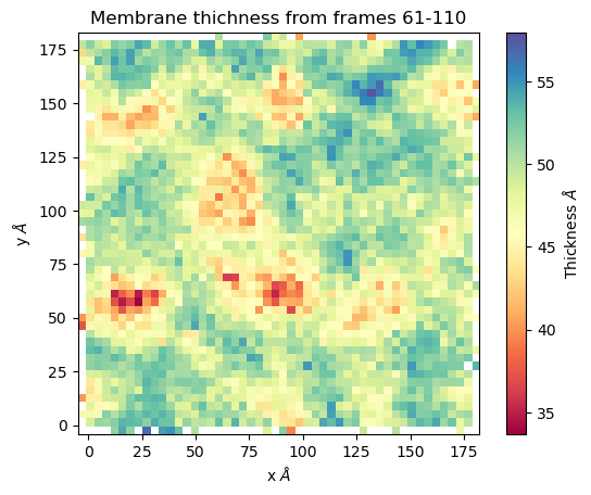

Membrane order parameters

The computation of order parameters is as easy as the computation of thickness. In this case you can also choose which layer the analysis will run (top, bot, both). Follows an example of running order parameters

scd_top, edges = membrane.thickness( "top",       # top layer
                                    50,           # nbins
                                    start = 61,   # Initial frame
                                    final = 110,  # Final Frame
                                    step = 1,     # Frames to skip
                                    )

scd_bot, edges = membrane.thickness( "bot",       # bot layer
                                    50,           # nbins
                                    start = 61,   # Initial frame
                                    final = 110,  # Final Frame
                                    step = 1,     # Frames to skip
                                    )

Now we can plot the results

from mpl_toolkits.axes_grid1 import make_axes_locatable
# Plot
fig, ax = plt.subplots(1,2, sharex = True, sharey = True)
first = ax[0].imshow(scd_top, extent=edges, cmap="Spectral")
ax[0].set_xlabel("x $\AA$")
ax[0].set_ylabel("y $\AA$")
ax[0].set_title("Top layer")
divider1 = make_axes_locatable(ax[0])
cax1 = divider1.append_axes("right", size="5%", pad=0.05)
cbar = fig.colorbar(first, cax = cax1)
# Point to a low ordered region
ax[0].add_patch(patches.Rectangle((48, 98), 20,20, linewidth = 1, edgecolor = "black", facecolor = "none"))
# High ordered region
ax[0].add_patch(patches.Rectangle((90, 120), 20,20, linewidth = 1, edgecolor = "black", facecolor = "none"))



second = ax[1].imshow(scd_bot, extent=edges, cmap="Spectral")
ax[1].set_xlabel("x $\AA$")
ax[1].set_title("Bot layer")
divider2 = make_axes_locatable(ax[1])
cax2 = divider2.append_axes("right", size="5%", pad=0.05)
cbar = fig.colorbar(second, cax = cax2)
cbar.set_label('|SCD| $\AA$')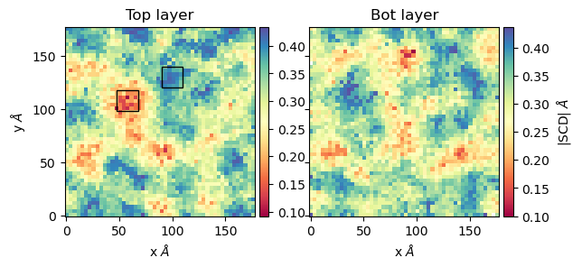

Here we highligted regions where the order parameters are low (red region) and high (blue region). From this region the lipids looks as follows

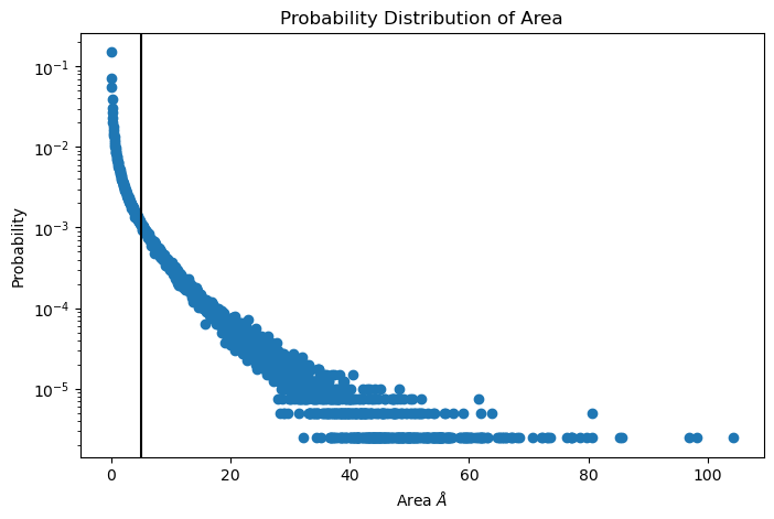
Packing defects

Packing defects is metric to evaluate the exposure of the hydrophobic core. It changes with membrane composition and also when proteins interact with the membrane. The computation of packing defects with packmemb implies extracting pdb files from the trajectories and then procesing them, which is time comsuming. Here we present an easy way to compute packing defects by only providing the trajectory and the topology file. Also, our code outperforms packmemb, doing the computations faster.

The packing defects code is the following:

# Compute deffects for the first frame
defects, defects_dict = membrane.packing_defects(layer = "top",         # layer to compute packing defects
                                                edges=[10,170,10,170],  # edges for output
                                                nbins = 400,            # number of bins
                                                )

# Plot defects
%matplotlib inline
plt.imshow(defects, cmap = "viridis", extent = defects_dict["edges"])
plt.xlabel("x  $[\AA]$")
plt.ylabel("y  $[\AA]$")
plt.show()

For various frames to get statistics

data_df, numpy_sizes = membrane.packing_defects_stats(nbins = 400,
                                                  layer = "top",
                                                  periodic = True,
                                                  start = 0,
                                                  final = -1,
                                                  step=1)

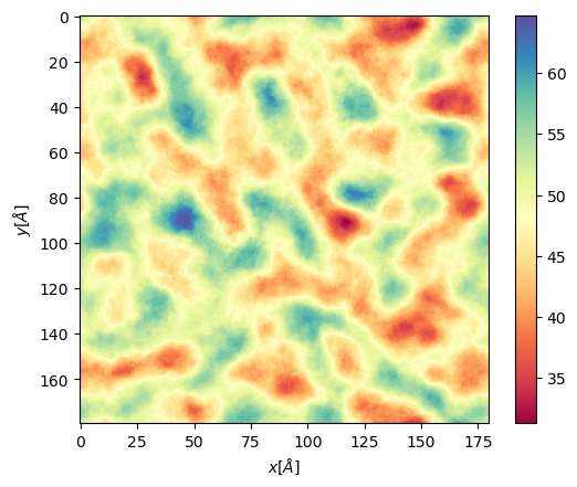
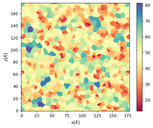
Area perlipid

We include the posibility of get Voronoi APL. For one frame can be obtained as follows:

voronoi_dict = membrane.voronoi_apl(layer = "top")

This return a dictionary that contains the areas per each lipid in the top bilayer

We can further map this voronoi to a twod grid and plot it

xmin = membrane.v_min
xmax = membrane.v_max
ymin = membrane.v_min
ymax = membrane.v_max
apl, edges = membrane.map_voronoi(voronoi_dict["points"], voronoi_dict["areas"], 180, [xmin, xmax, ymin, ymax])

plt.imshow(apl, extent = edges, cmap = "Spectral")
plt.xlabel("$x [\AA]$")
plt.ylabel("$y [\AA]$")
plt.colorbar()

For multiples frames:

resu, edges = membrane.grid_apl(layer = "top", start = 10, final = 100, step = 1, lipid_list = None)

plt.imshow(resu, extent = edges, cmap = "Spectral")
plt.xlabel("$x [\AA]$")
plt.ylabel("$y [\AA]$")
plt.colorbar()